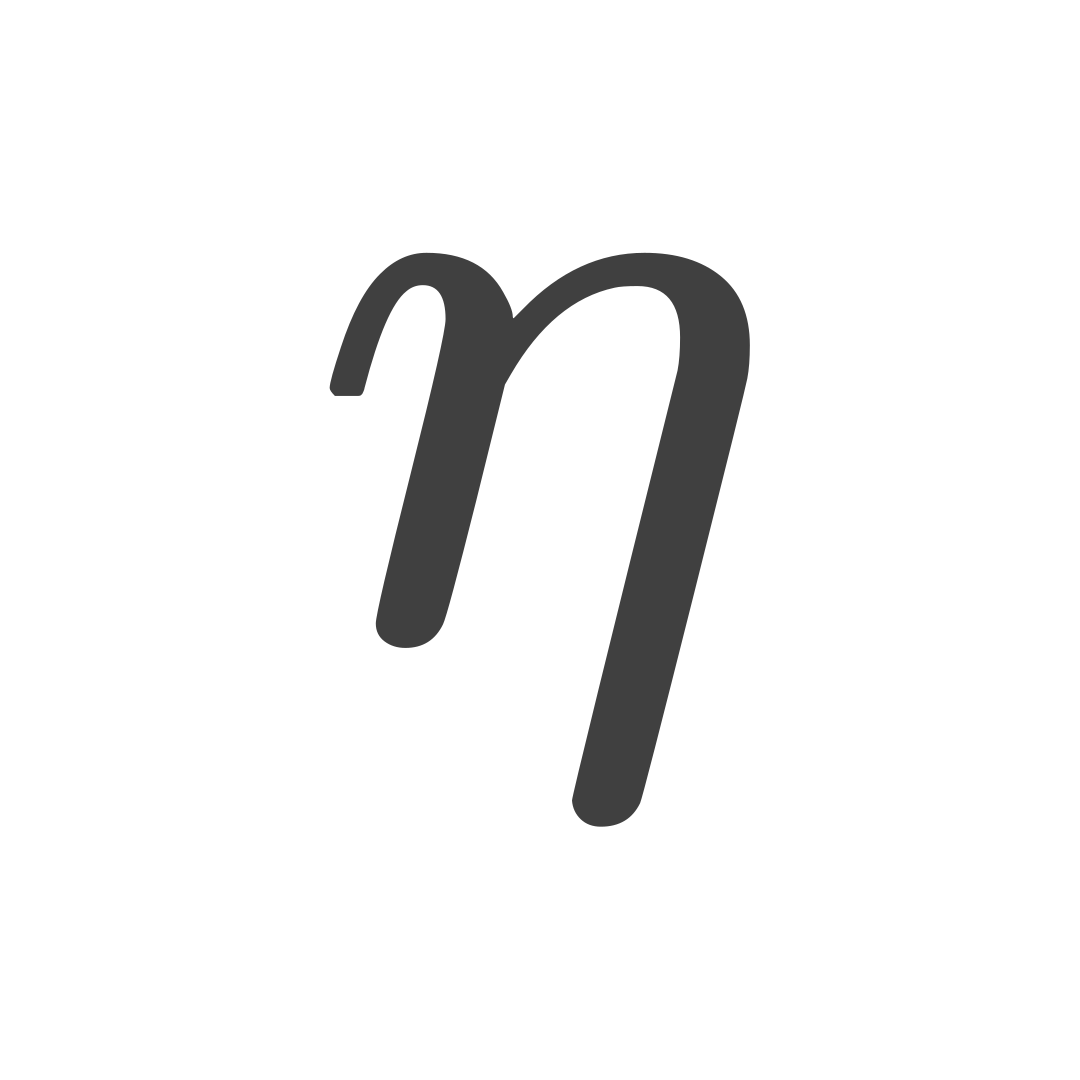
From Rectangular Strips to a Definite Integral
The familiar formulas for rectangles and triangles do not apply directly to a region with a curved boundary.
Definite integrals handle such regions by accumulating the areas of increasingly narrow strips. A Riemann sum partitions the interval, approximates each strip with a rectangle, and takes the limit of their total area.
Suppose a function bounds a region from to . We divide into subintervals of width .
Determining Area Using Definite Integrals
Use these three steps to calculate the area. Each step removes one source of error: the limits fix the interval, the integrand fixes the height, and the evaluation turns the antiderivative into a number.
Identify Integration Limits
The first step is to determine the lower and upper limits of integration. These limits indicate the range of values that bound the region whose area we want to calculate.
Determine the Integrand Function
The integrand describes the vertical height of the region. If throughout , the area is . If the graph crosses the axis, split the interval at its zeros or integrate so that every part contributes positive area.
Evaluate the Integral
After determining the limits and function, we can evaluate the integral using the fundamental theorem of calculus:
In this formula, is an antiderivative of .
Application to Quadratic Functions
Consider the region bounded by , the -axis, , and .
On , factor the function as . Every point in the interval satisfies and , so throughout the interval. The endpoint values and agree with this sign analysis.
Geometric area is nonnegative. Because the function is negative throughout this interval, its absolute value equals its negative, so:
Now evaluate the definite integral:
The area of that region is square units.
Application to a Radical Function
For a second example, calculate the area under from to .
The expression suggests substitution because the factor is proportional to the derivative of the expression inside the square root.
Set . Then , so .
The limits must use the same variable as the integrand: gives , while gives .
Now our integral becomes:
Here, and .
When using substitution in definite integrals, don't forget to change the integration limits according to the new substitution variable.
Exercises
Each problem describes a region bounded by curves and asks for its area, so the first step is to write down the bounds where the curves meet before you evaluate the integral.
-
Calculate the area of the region bounded by the curve , the -axis, and the lines and !
-
Determine the area of the region under the curve from to !
-
Calculate the area of the region bounded by the curve and the -axis!
Worked Solutions
-
First problem with function
Since this function is always positive, we can directly set up the integral:
After we integrate and evaluate, we obtain:
Therefore, the area of that region is square units.
-
Second problem with rational function
The antiderivative used in this integral is because its derivative is .
The area of that region is square units.
-
Third problem with parabola
First, find where the curve intersects the -axis:
So the intersection points are at and . Since this function is positive between these two points, we can directly integrate:
The area of that region is square units.