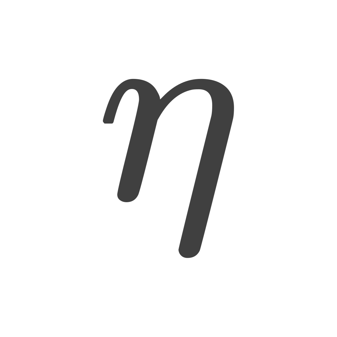
How Degree and Coefficients Shape a Polynomial Graph
The graph of a polynomial function provides a visual representation of how the function's value changes as the input value changes. The shape of this graph can vary greatly depending on the degree and coefficients of the function.
Point Plotting Method
One way to begin drawing a graph is to calculate several pairs that satisfy the function. The points guide the sketch, but a small table alone does not determine every feature of the graph. Roots, turning points, and end behavior provide additional checks.
Steps:
- Choose several different values for .
- Calculate the value for each chosen value.
- Create a table of value pairs.
- Plot these points on the coordinate plane.
- Connect the points with a smooth and continuous curve.
Linear Function Degree One
Graph the function .
We choose several values and calculate :
Plot the points and connect them:
Quadratic Function Degree Two
Graph the function .
Table of values:
Plot the points and connect with a smooth curve (parabola):
Cubic Function Degree Three
Graph the function .
Table of values:
Plot the points and connect with a smooth curve:
General Characteristics of Polynomial Graphs
Graphs of polynomial functions are always smooth (no sharp corners) and continuous (no jumps or breaks). Their general shape is heavily influenced by the degree of the polynomial.
- Degree : . The graph is a horizontal line.
- Degree : . The graph is a straight (slanted) line.
- Degree : . The graph is a parabola.
- Degree : . Its two ends point in opposite vertical directions, and it can have at most two turning points.
- Degree : The graph can have up to three 'peaks' or 'valleys'.
- Degree : The graph can have up to four 'peaks' or 'valleys'.
In general, the graph of a polynomial function of degree can intersect the -axis at most and has at most turning points (peaks or valleys).
End Behavior
The end behavior of a polynomial graph describes its direction as approaches positive infinity () or negative infinity ().
The end behavior is determined solely by the leading term :
- Degree (Even or Odd)
- Sign of the Leading Coefficient (Positive or Negative)
There are :
-
Even, (Positive):
-
As , (rises right )
-
As , (rises left )
-
Examples: ,
Graph of (Even, Positive)Graph rises to the left and right.
-
-
Even, (Negative):
-
As , (falls right )
-
As , (falls left )
-
Examples: ,
Graph of (Even, Negative)Graph falls to the left and right.
-
-
Odd, (Positive):
-
As , (rises right )
-
As , (falls left )
-
Examples: , ,
Graph of (Odd, Positive)Graph falls to the left and rises to the right.
-
-
Odd, (Negative):
-
As , (falls right )
-
As , (rises left )
-
Examples: ,
Graph of (Odd, Negative)Graph rises to the left and falls to the right.
-
Using End Behavior
The end behavior determines the directions of the graph's left and right ends without requiring a complete plot.
Application Example:
Match the following functions with their likely end behavior:
-
- Leading term:
- Degree (Even)
- Leading coefficient (Positive)
- End behavior: Rises left (), Rises right ()
Graph ofEnd Behavior: -
- Leading term:
- Degree (Odd)
- Leading coefficient (Negative)
- End behavior: Rises left (), Falls right ()
Graph ofEnd Behavior: -
- Leading term:
- Degree (Even)
- Leading coefficient (Negative)
- End behavior: Falls left (), Falls right ()
Graph ofEnd Behavior: -
- Leading term:
- Degree (Odd)
- Leading coefficient (Positive)
- End behavior: Falls left (), Rises right ()
Graph ofEnd Behavior:
By analyzing the leading term, we can predict the general shape of the graph at its ends.
Exercise
Consider
Determine its degree, leading coefficient, real zeros, behavior at each zero, and end behavior. Then describe the key features a correct sketch must show.
Worked Solution
The leading terms multiply to , so the polynomial has degree and leading coefficient .
The factored form gives the zeros directly:
- has multiplicity , so the graph crosses the -axis there.
- has multiplicity , so the graph touches the -axis and turns there.
Because the degree is odd and the leading coefficient is negative,
As one additional checkpoint, . A correct sketch therefore rises on the far left, crosses at , passes through , touches the axis at , and falls on the far right.